Cricket

old ipl project. Lots of suboptimal decisions date:2022-04-17 rendered: 2025-03-31

Code

# Load necessary libraries
# Using suppressPackageStartupMessages to keep output clean
suppressPackageStartupMessages({
  library(ggtext)
  library(lme4)
  library(tidyverse)
  library(plotly)
  library(viridisLite) # For better color scales
})

Indian Premier League

The goal of the present project is to download, clean, wrangle, and obtain insights from ipl data.

The data will be downloaded from cricsheet.org in a zip format. We will unzip the files to a directory.

Code

temp <- tempfile()
download.file("https://cricsheet.org/downloads/ipl_csv2.zip", temp)
unzip(zipfile = temp, exdir = "ipl_data") #takes a couple of minutes
rm(temp)

The next step would be load the data to R. We can achieve that using the read_csv function. However, while this data file is large and contains ball-by-ball details, it does not have match info i.e., who won the match and by how many wickets/runs.

We will obtain that data using the match info files. We can read only those files by adding them as a list for now.

Code

df <- read_csv("ipl_data/all_matches.csv") # read the data
files <- list.files(path = "ipl_data", pattern = "*_info.csv") #load the paths of
#metadata files ----
files <- paste0("ipl_data/", files) #append

One issue is that there are hundreds of files that match our pattern, and it is not possible to load them and use them effectively if we do it manually. One solution is to write a function that takes each of the file, appends it to a dataframe.

Code

f1 <- function(x) {
  y <- read.table(files[x], #load file
                  sep = ",",
                  skip = 2,
                  col.names = paste0("V",seq_len(5)), fill = TRUE)
  y <- y[,-1] #remove the first column 'info'

  y <- y %>% group_by(V2) %>% #number the column so that it can be pivoted wo errors
    mutate(id = seq_along(V2)) %>%
    ungroup() %>%
    mutate(V2 = paste0(.$V2, .$id)) %>%
    select(1, 2)

  y <- pivot_wider(y, names_from = V2, values_from = V3) %>% # lay data on side
    mutate(match_id = parse_number(file.path(files[x]))) %>%
    select(!starts_with(c("player","regis")))
  # the info file doesn't contain the match id! Parsing it from file names
}

df_info <- f1(1) # read the (meta)data file one
df_info <- df_info[FALSE, ] #keep only the headers
for (i in 1:length(files)) {
  X <- f1(i)

  df_info <- bind_rows(df_info, X)

}

df_info <- df_info %>% 
  rename_with(~str_remove(., "1")) %>%
  select(match_id, match_number, everything()) %>%
  select(!c(event, gender, venue)) %>%
  arrange(match_id)

Let’s take a look at the data frames we have so far.

Code

head(df)
head(df_info)

Code

final_df <- inner_join(df, df_info, by = 'match_id') # ugly but works..

#Clean up seasons
final_df <- final_df %>% 
    mutate(season.x = case_when(
        season.y == "2007/08" ~ '2008',
        season.y == "2009/10" ~ '2010',
        season.y == "2020/21" ~ '2020',
        TRUE ~ season.y),
        season.x = as.numeric(as.character(season.x))) 

#write.csv(final_df, "final_df.csv")
nanoparquet::write_parquet(final_df, "cricket/final_df.parquet") # 2025 change: saved 100x disk space

Load the final cleaned up data

Code

#final_df <- read.csv("final_df.csv")
final_df <- nanoparquet::read_parquet("cricket/final_df.parquet")

List of all teams that have played IPL so far

Code

(team_list <- final_df %>%
  distinct(team))

# A data frame: 19 × 1
   team                       
   <chr>                      
 1 Royal Challengers Bangalore
 2 Kings XI Punjab            
 3 Delhi Daredevils           
 4 Kolkata Knight Riders      
 5 Mumbai Indians             
 6 Rajasthan Royals           
 7 Deccan Chargers            
 8 Chennai Super Kings        
 9 Kochi Tuskers Kerala       
10 Pune Warriors              
11 Sunrisers Hyderabad        
12 Gujarat Lions              
13 Rising Pune Supergiants    
14 Rising Pune Supergiant     
15 Delhi Capitals             
16 Punjab Kings               
17 Lucknow Super Giants       
18 Gujarat Titans             
19 Royal Challengers Bengaluru

Exploring the Data

Lets start by making a function that gives some basic details about any given team

Code

team_stat <- function(team_name) {

f1 <- final_df %>% #_team_select
    group_by(season.x) %>%
    arrange(desc(match_id)) %>%
    filter(grepl(team_name, team, ignore.case = T) |
             grepl(team_name, team2, ignore.case = T))

f2 <- distinct(.data = f1, match_id) %>% count() #match count

f3 <- filter(f1, grepl(team_name, winner, ignore.case = T)) %>%#winning matches
    distinct(match_id) %>% count()

f4 <- filter(f1, grepl(team_name, winner, ignore.case = T))

df <- inner_join(f2, f3, by = "season.x") %>%
  rename(matches = n.x, wins = n.y) %>%
  mutate(win_rate = round(wins/matches * 100))


df$team <- f4[1,36] # add a new column with the team name
df <- df %>% unnest(last_col()) %>% 
  rename(team = last_col()) %>% #rename the column
  ungroup() #ungroup the df

return(df)

}

This particular function takes regex input

Code

team_stat("hyd")

# A tibble: 12 × 5
   season.x matches  wins win_rate team               
      <dbl>   <int> <int>    <dbl> <chr>              
 1     2013      17     9       53 Sunrisers Hyderabad
 2     2014      14     6       43 Sunrisers Hyderabad
 3     2015      14     7       50 Sunrisers Hyderabad
 4     2016      17    11       65 Sunrisers Hyderabad
 5     2017      14     8       57 Sunrisers Hyderabad
 6     2018      17    10       59 Sunrisers Hyderabad
 7     2019      15     6       40 Sunrisers Hyderabad
 8     2020      16     8       50 Sunrisers Hyderabad
 9     2021      14     3       21 Sunrisers Hyderabad
10     2022      14     6       43 Sunrisers Hyderabad
11     2023      14     4       29 Sunrisers Hyderabad
12     2024      16     9       56 Sunrisers Hyderabad

Code

team_stat("delhi")

# A tibble: 17 × 5
   season.x matches  wins win_rate team          
      <dbl>   <int> <int>    <dbl> <chr>         
 1     2008      14     7       50 Delhi Capitals
 2     2009      15     9       60 Delhi Capitals
 3     2010      14     7       50 Delhi Capitals
 4     2011      14     4       29 Delhi Capitals
 5     2012      18    11       61 Delhi Capitals
 6     2013      16     3       19 Delhi Capitals
 7     2014      14     2       14 Delhi Capitals
 8     2015      14     5       36 Delhi Capitals
 9     2016      14     7       50 Delhi Capitals
10     2017      14     6       43 Delhi Capitals
11     2018      14     5       36 Delhi Capitals
12     2019      16     9       56 Delhi Capitals
13     2020      17     8       47 Delhi Capitals
14     2021      16     9       56 Delhi Capitals
15     2022      14     7       50 Delhi Capitals
16     2023      14     5       36 Delhi Capitals
17     2024      14     7       50 Delhi Capitals

Code

team_stat("giants") #vs

# A tibble: 4 × 5
  season.x matches  wins win_rate team                
     <dbl>   <int> <int>    <dbl> <chr>               
1     2016      14     5       36 Lucknow Super Giants
2     2022      15     9       60 Lucknow Super Giants
3     2023      15     8       53 Lucknow Super Giants
4     2024      14     7       50 Lucknow Super Giants

Code

team_stat("giant$")

# A tibble: 1 × 5
  season.x matches  wins win_rate team                  
     <dbl>   <int> <int>    <dbl> <chr>                 
1     2017      16    10       62 Rising Pune Supergiant

How did any single team perform over the years?

Code

plot_team <- function(x3){
p1 <- team_stat(x3)
ggplot(p1, aes(x = as.factor(season.x), y = win_rate, group = 1)) +
  geom_point() +
  geom_line() +
  scale_y_continuous(limits = c(0, 100))+
  labs(
    x = "Season",
    y = "Win Rate",
    title = paste(first(p1[1,5]), "over the years")) #grabs the name of the team
}

Performance of SRH(DC) over the years

Code

plot_team("hyd|deccan") %>% ggplotly()

Delhi

Code

plot_team("delhi") %>% ggplotly()

Performance of all the teams over the years

Code

team_list2 <- team_list %>% filter(!grepl("X", team)) # Remove KXIPunjab

d2 <- NULL # create a empty df for stats of all teams
for (i in 1:nrow(team_list2)) {
  d1 <- team_stat(word(team_list2$team[i], 1))
  d2 <- bind_rows(d2,d1)
}

p4 <- ggplot(d2, aes(x = season.x, y = win_rate, group = 1)) +
  geom_point() +
  geom_line() +
  facet_wrap(~team)+
  scale_y_continuous(limits = c(0, 100))+
  labs(
    x = "",
    y = "Win Rate",
    title = "Winning Rate of the teams over the years")

ggplotly(p4)

Which team has won the most matches?

Code

final_df %>%
  distinct(match_id,.keep_all = TRUE) %>%
  count(winner) %>%
  arrange(desc(n)) %>%
  head(5) %>%
  ggplot(aes(x = reorder(winner,desc(n)), y = n))+
  geom_col()+
  labs(
    x = "Team",
    y = "Number of Wins")+
  scale_x_discrete(label = function(x) str_trunc(x, 19))+
  scale_y_continuous(expand = c(0,0), limits= c(0, 200))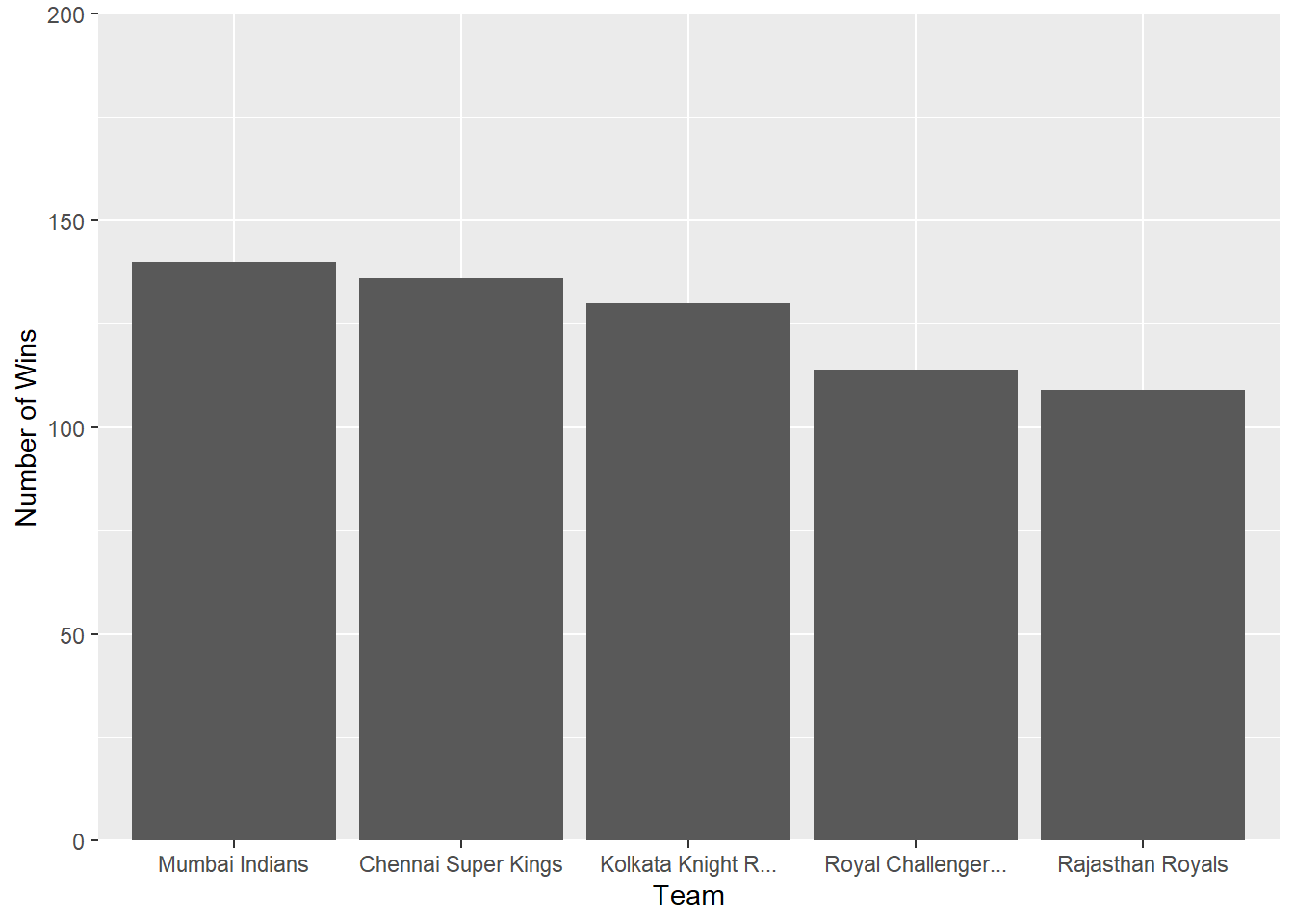

How many seasons has the IPL been going on for?

Code

ipl_season <- final_df %>%  
   distinct(season.x)
ipl_season %>% count()

# A data frame: 1 × 1
      n
  <int>
1    17

Lets write a function to get the top-scoring batmen of any given year

Code

high_scorer <- function(x = "", y = "", n = 10){
# x is a specific year
# y is a specific player
# n is the number of results to show
  y1 <- final_df %>%
    filter(grepl(x, season.x) & grepl(y, striker, ignore.case = T)) %>%
    group_by(striker) %>%
    summarise(runs = sum(runs_off_bat)) %>%
    arrange(desc(runs)) %>%
    head(n)


  y1 <- y1 %>% mutate(rank = row_number(), year = x) %>%
    select(3,2,1,4) %>% ungroup()

  #write a loop to generate boundaries, averages etc. for each batsmen?

  bound <- NULL
  for (i in min(y1$rank):max(y1$rank)) {
    striker_interest <- y1$striker[i]

    df_interest <- final_df %>% filter(grepl(x, season.x) &
                                         striker %in% striker_interest)

    sixes <- df_interest %>%
      group_by(striker) %>%
      filter(runs_off_bat == 6) %>%
      count() %>%
      ungroup() %>%
      rename(sixes = n)

    fours <- df_interest %>%
      group_by(striker) %>%
      filter(runs_off_bat == 4) %>%
      count() %>%
      ungroup() %>%
      rename(fours = n)

    fifties <- df_interest %>%
      group_by(striker, match_id) %>%
      summarise(runs = sum(runs_off_bat)) %>%
      filter(runs >= 50) %>% count() %>% ungroup() %>%
      rename(fifties = n)

    hundreds <- df_interest %>%
      group_by(striker, match_id) %>%
      summarise(runs = sum(runs_off_bat)) %>%
      filter(runs >= 100) %>% count() %>% ungroup() %>%
      rename(hundreds = n)

    not_out <- final_df %>% filter(grepl(x, season.x)  &
                                     (striker %in% striker_interest |
                                        non_striker %in% striker_interest)) %>%
      filter(ball >= 19.6) %>%
      dplyr::distinct(match_id) %>%
      count() %>%
      rename(not_out = n) %>%
      mutate(striker = striker_interest)#number of times not out

    runs <- df_interest %>%
      summarise(runs = sum(runs_off_bat)) %>%
      mutate(striker = striker_interest)

    matches <- final_df %>% filter(grepl(x, season.x)  &
                                     (striker %in% striker_interest |
                                        non_striker %in% striker_interest)) %>%
      dplyr::distinct(match_id) %>%
      count() %>%
      rename(matches = n) %>%
      mutate(striker = striker_interest)

    row_df <-  reduce(list(matches, fours, sixes, fifties, hundreds, not_out, runs), left_join, by = 'striker')

    row_df <- row_df %>% mutate(avg = round(runs/(matches - not_out), 2)) %>%
      select(-runs)

    bound <- bind_rows(bound, row_df)

    bound <- bound %>% replace(is.na(.), 0)

  }
  y1 <- left_join(bound, y1, by = 'striker')

  y1 <- y1 %>% select(11, 9, 2, 1, everything())

  if (y == "") {
  y1 <- y1 # if there is an empty value, then this changes the rank column
  } else {
 y1 <- y1 %>% mutate(rank = NA) 
  }
  
    if (x >= 2008) {
  y1 <- y1 # if there is an empty value, then this changes the year column
  } else {
 y1 <- y1 %>% mutate(year = NA) 
}
  
  return(y1)
}

This function takes year, name of player, and number of entries to return as the input

Code

high_scorer(x = 2024, y = , n = 5) # another change in 2025

# A data frame: 5 × 11
   year  rank striker   matches fours sixes fifties hundreds not_out   avg  runs
  <dbl> <int> <chr>       <int> <int> <int>   <int>    <dbl>   <int> <dbl> <dbl>
1  2024     1 V Kohli        15    62    38       6        1       2  57     741
2  2024     2 RD Gaikw…      14    58    18       5        1       1  44.8   583
3  2024     3 R Parag        14    40    33       4        0       2  47.8   573
4  2024     4 TM Head        15    64    32       5        1       0  37.8   567
5  2024     5 SV Samson      15    48    24       5        0       2  40.8   531

Number of runs of the top scorers across the years

Code

# hs2 <- NULL
# for (i in min(ipl_season):max(ipl_season)) {
#   hs <- high_scorer(x = i)
#   hs2 <- rbind(hs2,hs)
# }
# 
# nanoparquet::write_parquet(hs2, "cricket/hs2.parquet")
hs2 <- nanoparquet::read_parquet("cricket/hs2.parquet")

hs2 %>%
  filter(year >= 2011) %>%
  ggplot(aes(x = as.factor(rank),
             y = runs))+
  geom_col()+
  facet_wrap(~year)+
  labs(
    x = "",
    y = "Runs",
    title = "Total runs of the top 10 run scorers over the past seasons")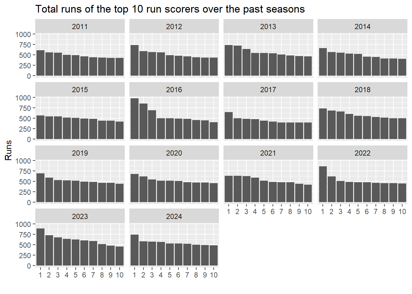

Some players have consistently been in the top-10 over multiple seasons. Though the trend seems to be decreasing. The top five runscorers repeat many times.

Code

(hs_freq <- hs2 %>% filter(year >= 2011) %>%
    count(striker) %>% arrange(desc(n)) %>% head(5))

# A data frame: 5 × 2
  striker       n
* <chr>     <int>
1 V Kohli       9
2 S Dhawan      8
3 DA Warner     7
4 KL Rahul      6
5 SK Raina      6

Let’s visualise this

Code

hs2 %>%
  left_join(hs_freq, by = "striker") %>%
  mutate(is_hs = ifelse(n > 0, '1', '0')) %>%
  filter(year >= 2011) %>%
  ggplot(aes(x = as.factor(rank),
             y = runs,
             fill = is_hs))+
  geom_col()+
  facet_wrap(~year)+
  labs(
    x = "",
    y = "Runs",
    title = "<b style='color:#f8766d'>Top five</b> most runscorers
             perform consistently.")+
  theme(plot.title = element_markdown(),
        legend.position = "none")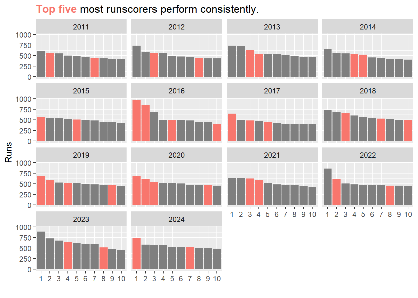

Are first innings runs increasing over the years?

We can visualise this by plotting runs in the first innings and matches from the beginning of IPL

Code

first_innings_run <- final_df %>%
  mutate(runs = rowSums(select(.,runs_off_bat,extras), na.rm = TRUE)) %>%
  group_by(match_id, innings) %>%
  summarise(total_runs = sum(runs)) %>%
  filter(innings == 1) %>%
  left_join(.,final_df,by = 'match_id') %>%
  distinct(match_id, .keep_all = TRUE) %>%
  ungroup() %>%
  mutate(match_no = row_number()) %>%
  select(match_no, everything())

p2 <- first_innings_run %>%
  ggplot(aes(x = match_no, y = total_runs))+
  geom_point(aes(color = as.factor(season.x))) +
  geom_smooth(method = "lm")+
  guides(color = guide_none())+
  labs(
    x = "Matches",
    y = "Number of runs in first innings",
    title = "Noticeable increase in the runs (Hover for more details)"
  )

ggplotly(p2)

What about boundaries (4s and 6s)

Code

boundaries <- final_df %>% 
    group_by(match_id, runs_off_bat) %>% 
    count(runs_off_bat) %>% filter(runs_off_bat == 4 | runs_off_bat == 6 ) %>%
  ungroup() %>% 
  mutate(match_no = row_number()) %>%
  select(match_no, everything())

p5 <- boundaries %>% 
    inner_join(.,first_innings_run, by = 'match_id') %>% 
    ggplot(aes(x = match_no.y, y = n, color = as.factor(runs_off_bat.x))) +
    geom_point()+
    geom_smooth()+
    labs(
        x = "Matches",
        y = "Number of boundaries per match",
        title = "Boundaries and IPL matches",
        col = "4/6"
    )
ggplotly(p5)

Stats

A simple linear model for testing for increase in runs over time

Code

lm(total_runs ~ match_no, first_innings_run) %>% summary()


Call:
lm(formula = total_runs ~ match_no, data = first_innings_run)

Residuals:
     Min       1Q   Median       3Q      Max 
-108.533  -19.091   -0.118   21.021  108.646 

Coefficients:
             Estimate Std. Error t value Pr(>|t|)    
(Intercept) 151.67752    1.87866  80.737   <2e-16 ***
match_no      0.02531    0.00297   8.523   <2e-16 ***
---
Signif. codes:  0 '***' 0.001 '**' 0.01 '*' 0.05 '.' 0.1 ' ' 1

Residual standard error: 31.06 on 1093 degrees of freedom
Multiple R-squared:  0.06232,   Adjusted R-squared:  0.06146 
F-statistic: 72.64 on 1 and 1093 DF,  p-value: < 2.2e-16