pretty map

Code
# Create a pretty map using OpenStreetMap data
# Adapted from: http://estebanmoro.org/post/2020-10-19-personal-art-map-with-r/
# Date: 2020-10-26
# Last rendered: 2025-03-31

# Load required packages
library(osmdata)
library(sf)
library(ggplot2)

# Get bounding box. Use Key:official_name from OSM for accurate details
bbx <- getbb("Hyderabad District")

# Define min/max coordinates for the map boundaries
min_lon <- bbx[1, 1]
max_lon <- bbx[1, 2]
min_lat <- bbx[2, 1]
max_lat <- bbx[2, 2]

# Big roads
highways <- bbx |>
  opq(timeout = 180) |>
  add_osm_feature(
    key = "highway",
    value = c(
      "motorway", "trunk", "primary", "secondary", "tertiary",
      "motorway_link", "trunk_link", "primary_link",
      "secondary_link", "tertiary_link"
    )
  ) |>
  osmdata_sf()

# Preview
ggplot() +
  geom_sf(
    data = highways$osm_lines,
    aes(color = highway),
    size = 0.4,
    alpha = 0.65
  ) +
  theme_void()


# Small roads
streets <- bbx |>
  opq(timeout = 180) |>
  add_osm_feature(
    key = "highway", 
    value = c(
      "residential", "living_street", "service", "unclassified",
      "pedestrian", "footway", "track", "path"
    )
  ) |>
  osmdata_sf()

# Lotsa streets
ggplot() +
  geom_sf(
    data = streets$osm_lines,
    aes(color = highway),
    size = 0.4,
    alpha = 0.65
  ) +
  theme_void()

color_roads <- rgb(0.42, 0.449, 0.488)

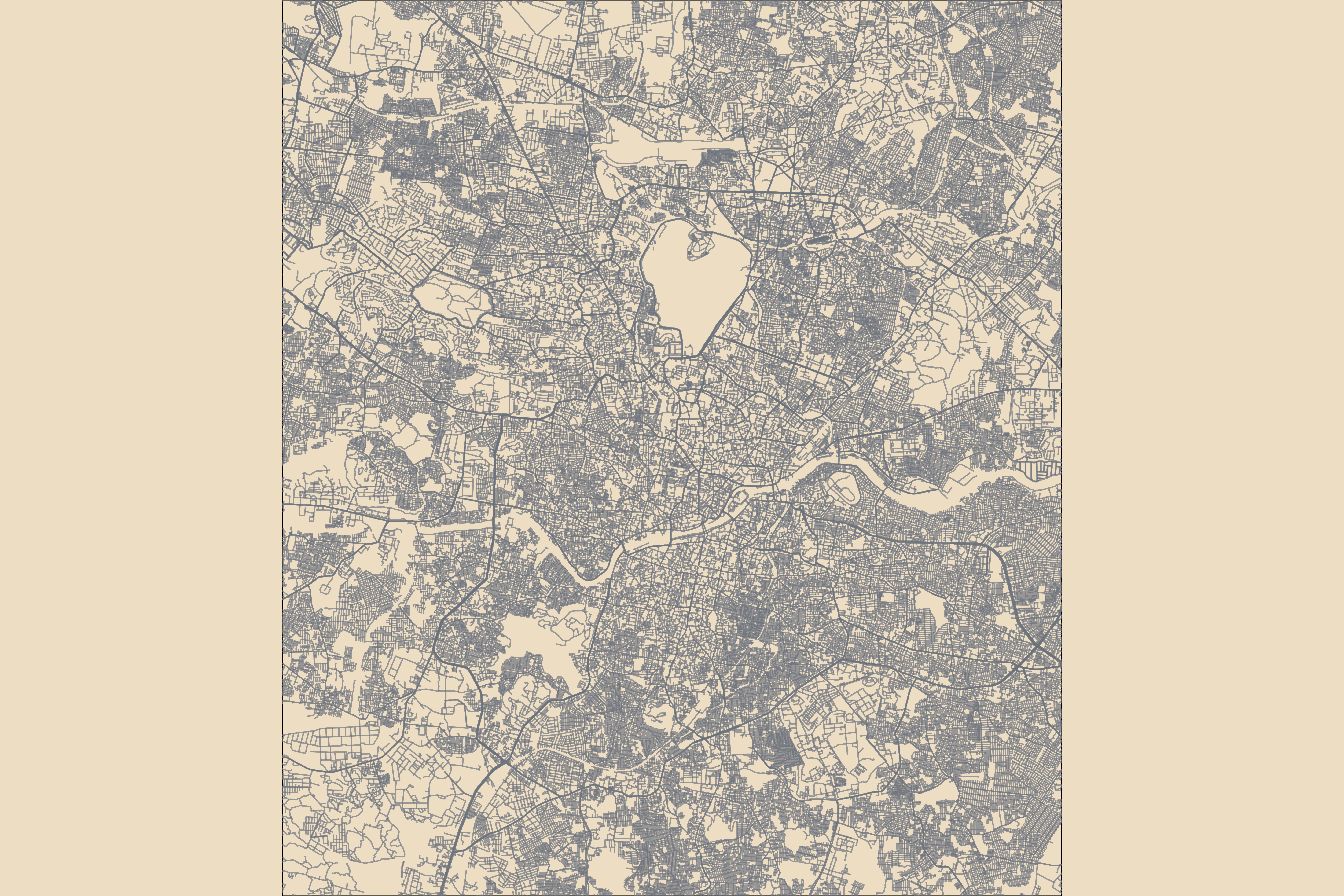
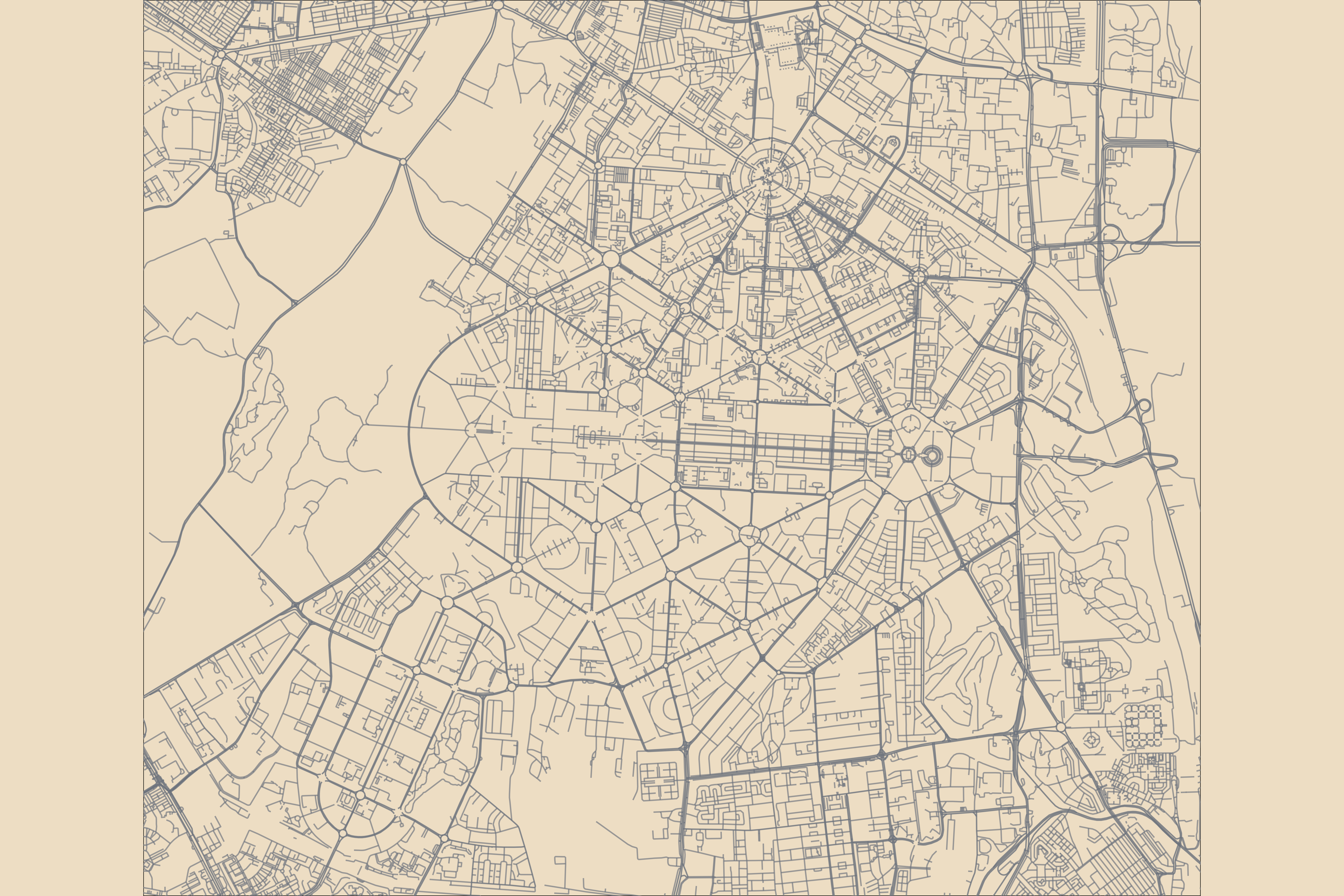
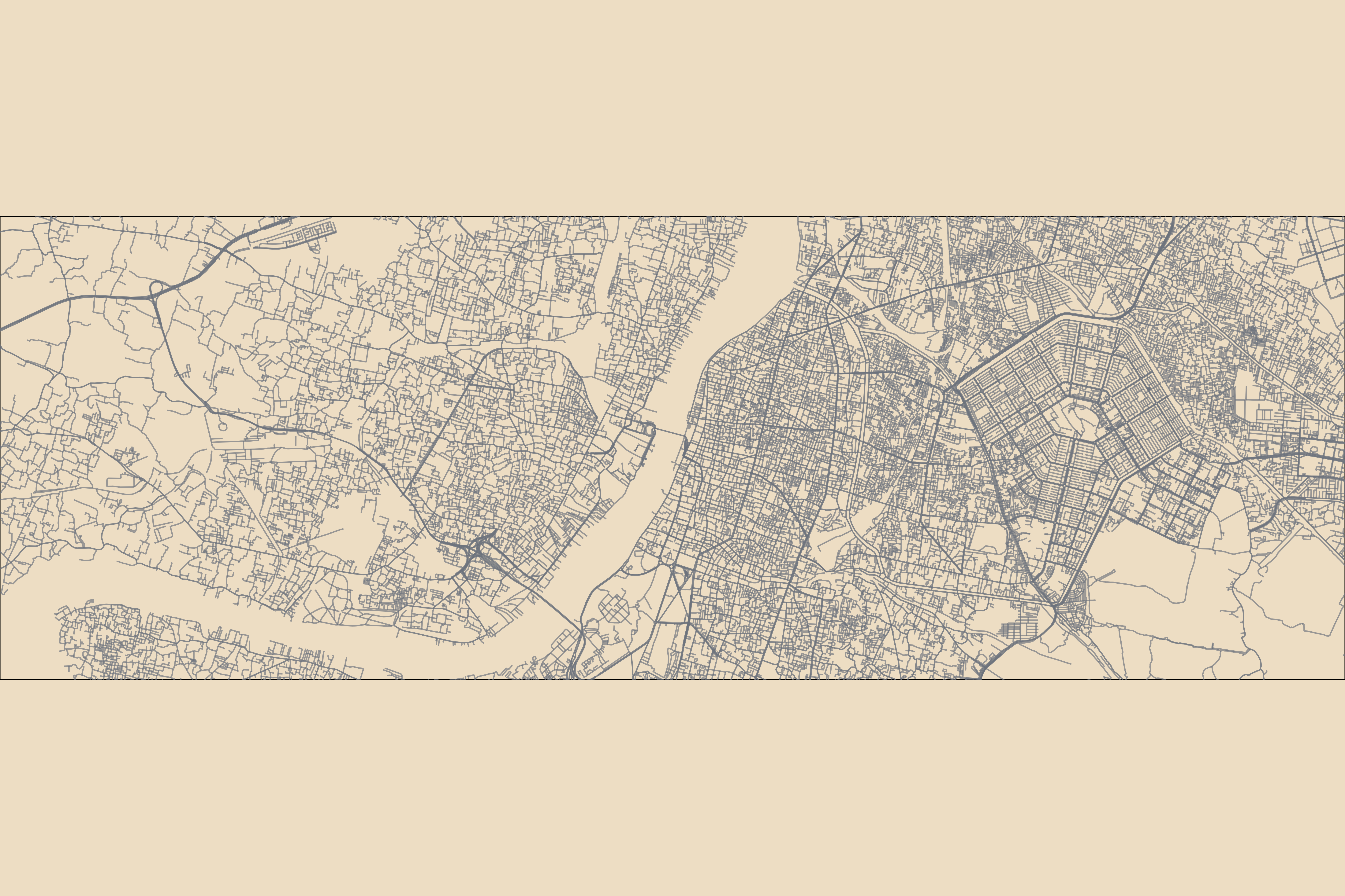
# Create final map
final_map <- ggplot() +
  geom_sf(
    data = streets$osm_lines,
    col = color_roads,
    size = 0.4,
    alpha = 0.65
  ) +
  geom_sf(
    data = highways$osm_lines,
    col = color_roads,
    size = 0.6,
    alpha = 0.8
  ) +
  coord_sf(
    xlim = c(min_lon, max_lon),
    ylim = c(min_lat, max_lat),
    expand = FALSE
  ) +
  theme_void() +
  theme(
    legend.position = "none",
    plot.background = element_rect(fill = "#edddc3")
  )

# Save the map
ggsave(
  filename = here::here("projects/map/hyd.png"),
  plot = final_map,
  width = 36, 
  height = 24, 
  units = "cm",
  dpi = 500
)